From Waveforms to Tokens: Exploring Residual Vector Quantization

At my audio ML research work with verda.ai, I come across several interesting deep learning and signal processing concepts. One idea that stands out for being both powerful and surprisingly intuitive is Residual Vector Quantization (RVQ). This method transforms continuous signals like audio waveforms into discrete tokens—similar to how language is broken down into words or characters. What makes RVQ particularly fascinating is how it achieves high-precision representation through iterative refinement—a concept I first encountered while working with Encodec, a neural audio codec developed by Meta AI. Beyond audio compression, these tokenized representations unlock advanced machine learning applications across diverse domains. In this post, I'll walk through the core ideas of RVQ, examine its implementation in Encodec, and show how I'm adapting these principles for earthquake signal analysis.

Understanding Residual Vector Quantization

Before diving into RVQ, let's consider the challenge of representing continuous signals like audio. These signals often contain considerable redundancy—imagine a repeating pattern in a musical note, where the same waveform cycle is captured hundreds of times per second. Recording every tiny fluctuation isn't always necessary for human perception or practical applications. For instance, CD-quality audio captures 44,100 samples per second at 16 bits per channel in stereo, generating approximately 10.6 megabytes per minute. This data can contain redundancies, which might lead to less efficient storage and processing.

To address this challenge, we need a method that captures the significant characteristics of these signals in a more compact and efficient form. Vector quantization (VQ) approaches this by creating a finite set of reference patterns or representatives that can approximate the original data with acceptable fidelity.

The Analogy: From Colors to Tokens

Imagine we're tasked with cataloging the colors of every marble in a massive collection. Each marble's color starts as a continuous spectrum of reflected light, which can be measured and represented as a point in 3D space using standard RGB coordinates - much like how digital cameras and screens represent colors. In typical digital systems, each RGB channel uses 8 bits (values 0-255), requiring 24 bits total per marble.

While this digital representation is already a form of discretization from the continuous spectrum of light, it still requires considerable storage space when dealing with large collections. But what if we wanted to compress this even further? Instead of using the full range of RGB values, we could create a smaller palette of standard reference colors—let's say 16. Then, for each marble, you find the closest matching color in your palette and record its index (e.g., "color 7"). This way, we've reduced a 24-bit color representation down to just 4 bits (since 2⁴ = 16).

This is the essence of vector quantization (VQ): breaking a high-dimensional space into discrete regions, each represented by a reference value. The process works as follows:

Codebook Creation: Choose a set of reference colors to form your "codebook."
Space Division: Divide the entire color space into regions, each corresponding to one of the reference colors.
Vector Assignment: For each marble, find the closest reference color and record its index (or "token").

By using this palette approach, we've compressed the information significantly. Instead of storing RGB values (24 bits per marble), we now only need to store the index of the reference color (4 bits for 16 colors). Each index corresponds to a token, effectively tokenizing the color space into discrete units. However, single-level quantization often loses important details.

Enter Residual Vector Quantization

Instead of trying to capture everything with one set of reference vectors, residual vector quantization (RVQ) works in stages:

Initial Quantization:
- Start with a basic codebook (e.g., 16 main colors).
- Approximate each data point using the nearest centroid from this codebook.
- Record the index (token) of the selected centroid.
Compute Residuals:
- For each data point, calculate the residual—the difference between the original vector and its approximation from the first level.
- These residuals represent details missed in the initial quantization.
Secondary Quantization:
- Create a second codebook to quantize these residuals.
- Approximate each residual with the nearest centroid in the second codebook.
- Record the index (token) of the selected centroid.
Iterative Refinement:
- Repeat the process with additional codebooks to capture finer details.

The final approximation of each data point is the sum of the approximations from all quantization levels:

Approximation = Centroid₁ + Centroid₂ + ... + Centroidₙ

Each centroid index serves as a token, and combining these tokens across levels forms the tokenized representation of the original data point.

This method effectively converts complex, continuous data into sequences of discrete tokens that can be efficiently stored, transmitted, and processed.

For a deeper dive into the details of RVQ, I recommend reading Dr. Scott H. Hawley's excellent blog post.

Encodec: RVQ in Neural Audio Compression

Autoencoders are neural networks that learn to compress and reconstruct data through a bottleneck layer, leveraging nonlinear transformations to capture complex patterns. Applying RVQ in this learned latent space takes compression a step further, converting continuous latent vectors into discrete tokens while preserving the richness of the nonlinear encoding.

Encodec, developed by Meta AI, demonstrates how powerful this approach can be for audio compression. Let's examine its 24 kHz mono configuration to understand how these principles work in practice. The system produces a latent vector for every 320 consecutive time samples of the input audio, which is then quantized and later decoded back to audio.

The Encodec Architecture

The system comprises three main components:

Encoder Network:
- Input: Mono audio sampled at 24 kHz
- Process: Transforms the waveform through convolutional and LSTM layers
- Output: Produces a 128-dimensional latent vector for every 320 samples in the audio stream (13.33 ms)
Residual Vector Quantization (RVQ):
- Quantization Levels: Multiple codebooks are used iteratively
- Codebooks: Each contains 1024 centroids, requiring 10 bits per centroid index
- Tokens: Each level's centroid index serves as a token
- Final Representation: Sequence of tokens from all codebook levels for each latent vector
Decoder Network:
- Input: Quantized latent vectors (token sequences)
- Process: Reconstructs the audio waveform
- Output: Reconstructed audio signal

Understanding the Compression

Frames and Tokens

Frames per Second:
- Sample Rate: 24,000 samples/sec
- The encoder produces one latent vector for every 320 samples in the audio stream
- Latent Vectors per Second: 24,000 ÷ 320 = 75
Tokens per Frame:
- Each latent vector is quantized using multiple codebook levels
- Each codebook level produces one token
- Number of tokens per latent vector equals the number of codebook levels used

Bitrates and Compression Ratios

Encodec offers multiple bitrates by adjusting the number of codebook levels. The compression works as follows:

Each codebook level requires 10 bits (from 1024 centroids)
Total bits per latent vector = Number of codebook levels × 10 bits
Bits per second = Total bits per latent vector × 75 vectors/sec
Original audio bitrate: 24,000 samples/sec × 16 bits/sample = 384,000 bits/sec (384 kbps)
Compression ratio = 384,000 ÷ (Bits per second)

For example, in 6 kbps mode:

Using 8 codebook levels: 8 × 10 bits = 80 bits per latent vector
Bitrate: 80 bits × 75 vectors/sec = 6,000 bits/sec
Resulting in a compression ratio of 64:1 (384,000 ÷ 6,000)

Looking at the compression more closely:

Original 320 samples require: 320 samples × 16 bits = 5,120 bits
When compressed to 1.5 kbps (2 codebook levels): 2 × 10 bits = 20 bits
This achieves a compression ratio of 256:1 (5,120 ÷ 20)

Listen and compare how these different compression levels affect audio quality on Meta AI's official Encodec demonstration page.

Beyond Compression: Transforming Signals into Deep Learning Tokens

While RVQ originated in compression research, researchers discovered its potential for deep learning when exploring efficient ways to process continuous signals. The technique's iterative quantization transforms complex waveforms into discrete sequences while preserving signal characteristics through successive refinements. These discrete representations align naturally with Transformers, which were designed for processing token sequences in language tasks. This compatibility allows researchers to adapt powerful sequence modeling techniques from natural language processing to continuous signal data.

Recent methods have leveraged these tokenized representations across audio processing tasks. Meta's AudioGen and MusicGen use EnCodec tokens for sound effects and musical composition. VoiceCraft demonstrates how these tokens enable both voice manipulation and speech synthesis without task-specific training. Google's AudioLM shows similar capabilities in speech and music generation. These successes in audio processing raise a broader possibility: could similar quantization approaches help analyze and process other continuous signals? From medical readings to geophysical signals, many fields work with complex waveform data that might benefit from these techniques.

From Audio to Earthquakes: Applications in Seismic Analysis

Inspired by audio quantization, I developed EQcodec by adapting Encodec's architecture for seismic waveforms. The figure demonstrates signal reconstruction across different quantization levels.

A central storage system in my laboratory houses over 10 TB of earthquake data. When training deep learning models, I need to access these files at gigabyte-per-second speeds for efficient processing, but our network throughput is limited to about 12 MB/s. While my workstation's SSD would provide the fast access needed for training, its ~1 TB of free space wouldn't fit the dataset I want to work with.

I trained a version of EQcodec at 40 Hz sample rate with four quantization levels, using 4080 centroids at each level. This configuration achieves approximately 26:1 compression, allowing the dataset to fit within the available SSD storage. Open-sourcing this model could enable systems with limited computational resources to participate in seismic signal analysis.

These tokenized representations also suggest possibilities for language modeling-inspired tasks in seismic analysis. I will present this work at the 1st Conference on Applied AI and Scientific Machine Learning (CASML 2024). See you there! (Update: You can find the poster I presented here.)

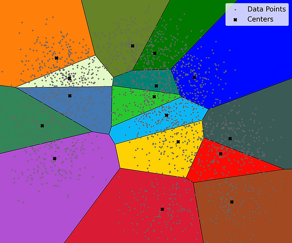
Figure: Vector quantization divides the color space into regions, with each region represented by a reference color (marked by black crosses).

Figure: Top: First-level quantization showing basic colors. Bottom: Second-level quantization showing finer color variations.

Figure: 3D visualization showing how RVQ represents vectors in space. Initial quantization vectors are shown in different colors.

Figure: Detailed view of how residual vectors (shown around limegreen) refine the initial approximation.

Figure: Snapshot of the Encodec Architecture as presented by Défossez et al. in their paper, 'High Fidelity Neural Audio Compression'.